Regression modelling is an important part of our everyday lives, whether we realise it or not. It informs websites about what ads to show us, and when. It forms the methodological basis for a number of academic studies across fields as diverse as economics, medicine, and psychology. In this article, I hope to give you a basic introduction to linear regression, how it works, as well as some of the issues surrounding its use. All while relying primarily on intuitive explanation.
1. What is regression?
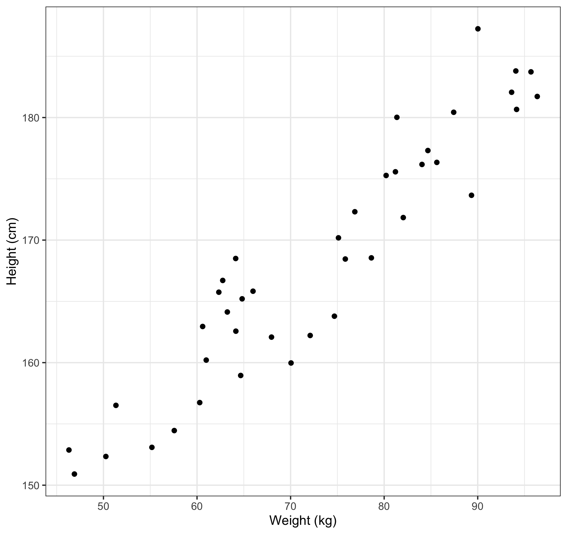
Regression is essentially putting a line of best fit through some data. Let’s say we have some data on people’s height (measured in cm) and weight (measured in kg), and we wanted to examine the relationship between the two. Now we could simply plot the data on a scatter plot and eyeball it. Let’s say the data looks like this:

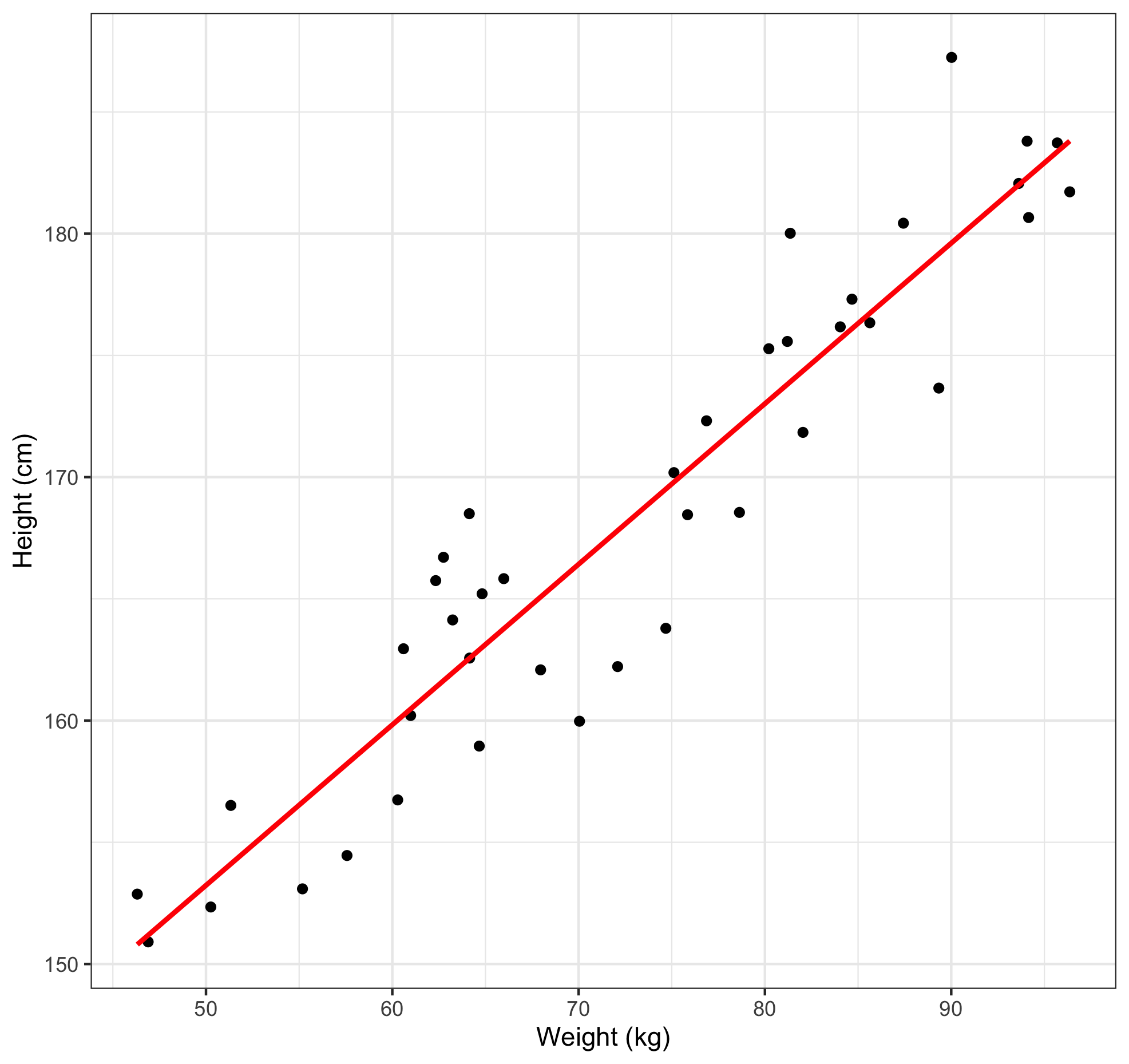
This clearly shows a positive linear relationship between height and weight. But what if we wanted to be more exact about this relationship? Well, we could just add a line of best fit, like so.

And there we have fitted a regression line. We can also describe this line mathematically with this formula:
But what does this mean? Well, this formula tells us what we should expect the height to be of any person given their weight. Let’s say that we know the weight of a given person, we could then use this formula to estimate what their height might be by simply filling in their weight. Let’s say that this person weighs 70 kgs, we can amend the formula above:
So, using our model, we estimate that this person is around 1.66 meters tall. What’s more, when we examine our data, we can see that there is a person who weighs around 70 kgs and measures up at around 1.59 meters tall. Not a bad prediction by our model.
2. How does regression work?
Single variable (univariate) linear regression equations typically take the following form:
So, let’s break this equation down piece by piece. ‘y’ represents the outcome we are trying to predict. In the previous example, we were trying to predict the people’s height, so height would be our outcome. ‘b’ is a constant value, consider this as our starting point for our prediction before considering anything else. In our previous example, in the unlikely event that we had a person who was weightless, our model would predict that they would be 1.22 meters tall. 'm' is an estimated parameter of the relationship between our variable of interest and our outcome. This can tell us about the size of the relationship, as well as whether this relationship is positive or negative. In the previous example we saw not only that the relationship was positive, but specifically that for every added kg of weight, our model predicted that our person would be 0.6595 cm taller.
But where did we get these numbers from?
The estimates for 'm' in the above model are derived using another formula called the 'Ordinary Least Squares' (OLS) formula, and looks like this:
| m = | ∑(x - x̅) * (y - y̅) |
| ∑(x - x̅) 2 |
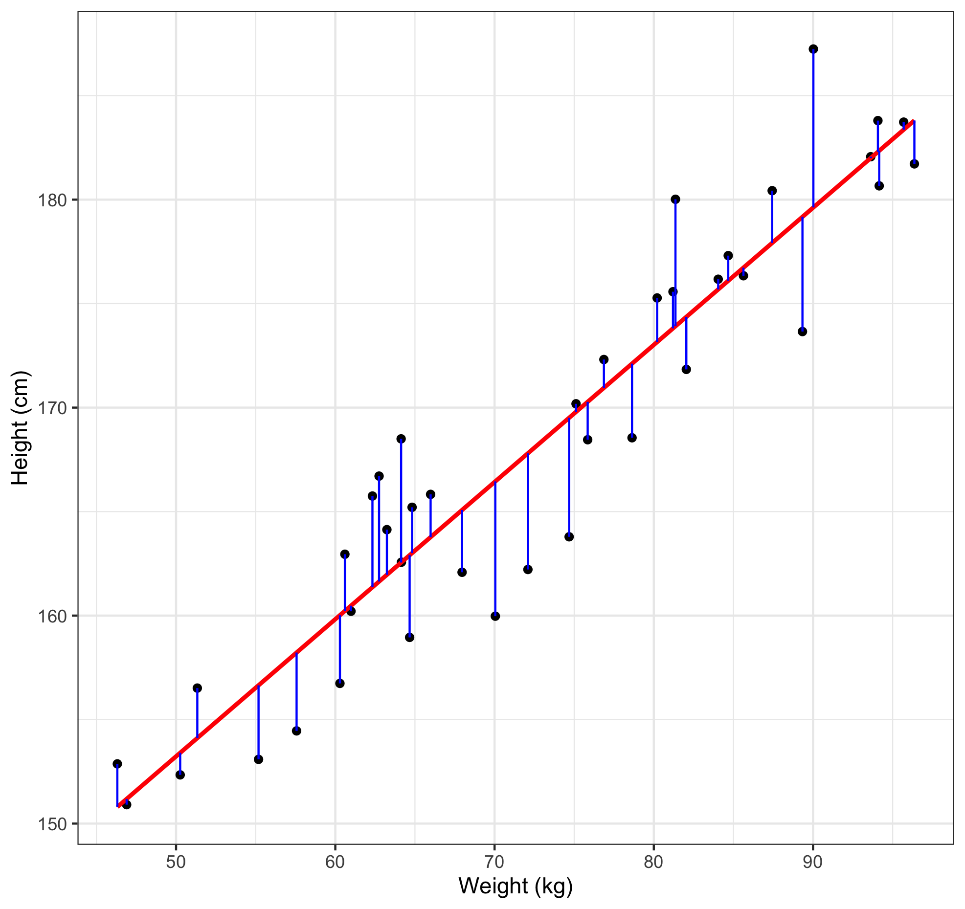
Don't worry if it looks complex, all this formula does is help us select the value of m such that the difference between the predicted values of y and the actual values of y are minimised. This process is called minimising the squared error. Why squared? Because squaring a difference will make it positive, so that a positive and negative error won't cancel each other out. Going back to our previous plot, we can plot the errors onto the graph in blue.

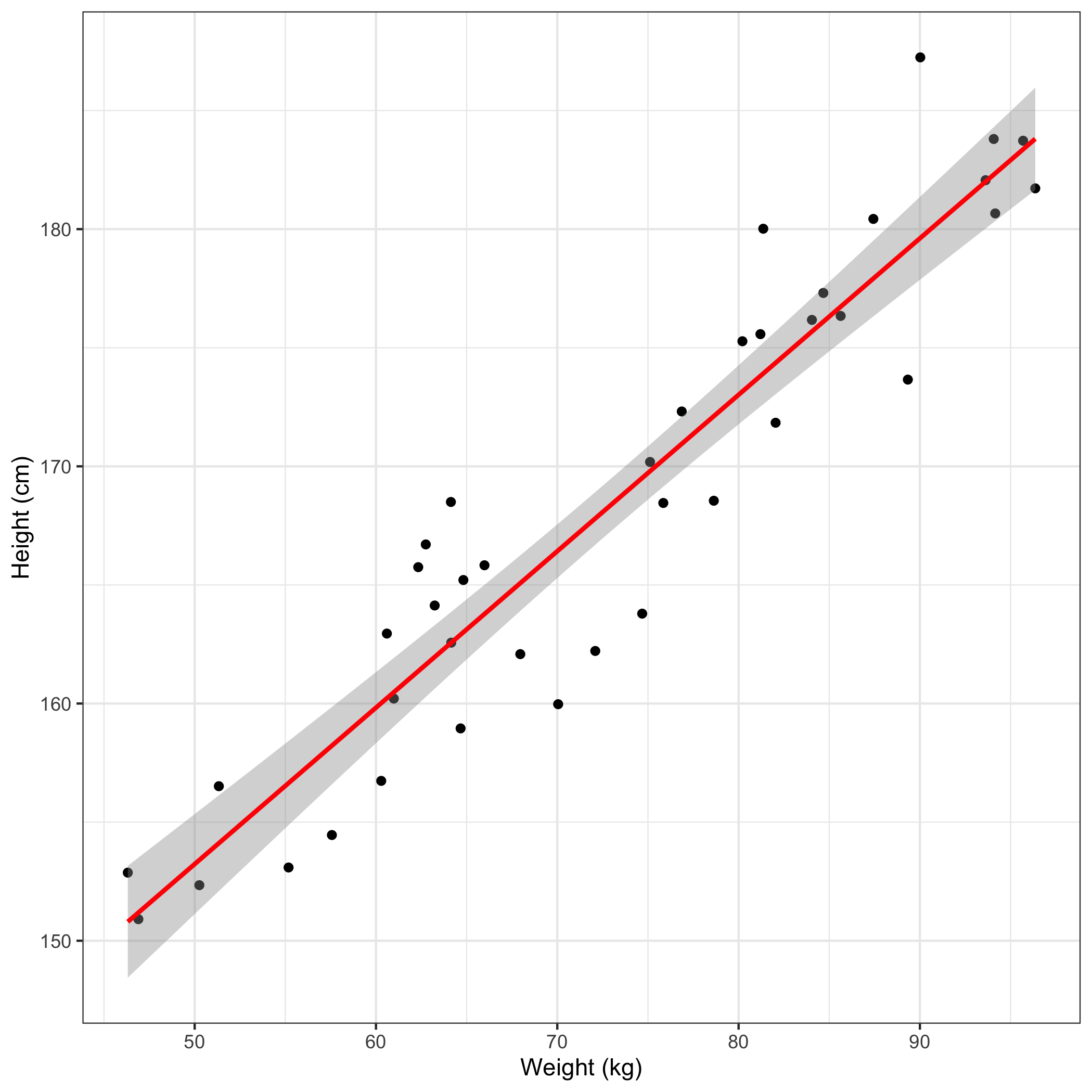
On the topic of errors, there is one final aspect of a regression equation that we have to discuss, this is the error term. So far we have been dealing with point estimates. These are the exact numerical estimates of our model. For example, our earlier prediction of 1.66 meters tall for a person who weighed 70 kgs was a point estimate. Our model also suggested that the height of this person could be 3.466 cm either side of that estimate. We can amend the earlier formula to account for this error:
Filling in the values from our model gives us the following model:
We can also plot this onto our graph to provide a visual representation.
